Interrupted Time Series Analysis for Quality Improvement Projects

Broadly speaking, quality improvement (QI) interventions are changes made to a system to improve its performance, aiming to increase the occurrence of a desirable event or decrease the occurrence of an undesirable one. I will refer to both as the “focal indicator.” Medical examples might include efforts to increase colon cancer screening in an office practice, or to decrease the incidence of central line infections in a hospital.

Pre/post designs are commonly used for analysis of QI interventions. A search on the PRiMER journal website for the text string “pre” co-occurring with “post” currently yields 60 results. Searching PubMed for “pre” and “post” and “quality improvement” currently produces nearly 4,000 citations.

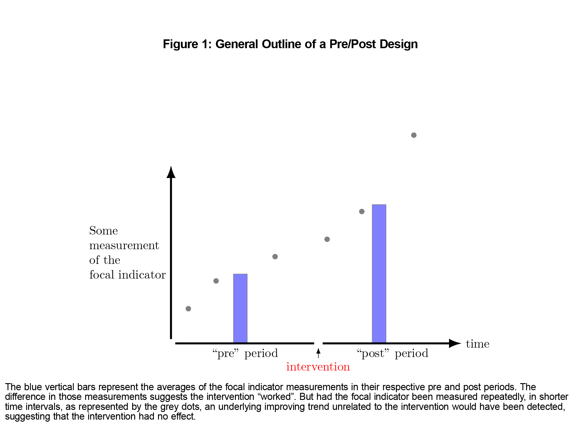
The blue vertical bars in Figure 1 illustrate the general outline of a pre/post design:

1. Measure the focal indicator during some arbitrary period of time. This “pre” period is sometimes referred to as a “historical control.” 
2. Launch the intervention.
3. Measure the focal indicator again during some arbitrary period of time. This “post” period is often, but needn’t be, the same length as the “pre.”
4. Compare the pre and post measurements, often with some sort of statistical hypothesis.

The measuring, both pre and post, could be done retrospectively (eg, chart review) or prospectively.

Although conceptually simple, this approach has several drawbacks, chief among them that time passes and things change, unrelated to the intervention. Staff, policies, procedures, epidemics, etc inevitably come and go. Any of these could influence the occurrence of the focal indicator and lead to the conclusion, possibly erroneous, that the QI intervention “worked.” Unlike pre/post designs, a time series of measurements can disclose and control for ongoing trends, such as the grey dots in Figure 1. Brady et al provide graphical examples of underlying trends confounding the conclusions drawn from simple pre/post studies.¹

A time series consists of repeated measurements of the same indicator at fixed intervals. Trends and autocorrelation are key features of time series that must be kept in mind during analysis.

Two common types of trends are secular and seasonal. Secular trends have also been called “rising tides.”² They represent overall long-term improvements independent of the particular QI initiative being implemented. Seasonal trends, such as the epidemiology of influenza, are familiar to physicians. Seasonal trends are also part of residency practices, where we hope that performance improves from July to June each year.

Much of classical statistical inference assumes that observations are independent of one another. However, time periods often are not: what happens this week in a medical practice or hospital may depend, to some degree, on what happened last week. This is known as “temporal autocorrelation.” If you know yesterday’s temperature, you have a fair, albeit imperfect, idea of what today’s temperature might be. Before the current period’s measurement is even obtained, something about it is already known, based on previous measurements. An autocorrelated data set contains less information overall than an uncorrelated sample of equal size, because each observation is conveying partially redundant information.

The results of a QI study can be interpreted on a variety of levels:

1. If the goal is simply to see if the focal indicator changed, then a rudimentary pre/post analysis (represented by the vertical blue bars in Figure 1) suffices. It allows assertions like, “The frequency of colon cancer screening among eligible patients was higher after we made the change than it was before.”
2. A more ambitious goal would be to associate the timing of the change with that of the intervention, controlling for trends.³ This is where ITS fits in. ITS analysis allows assertions like, “Central line infections started declining when we made the change.”
3. The boldest claim is that the intervention caused the change in the focal indicator. This generally requires a suitable control setting where the intervention was not implemented—a “usual care” setting. This can present significant operational, administrative, financial, and ethical challenges, but examples can be found.^4–6 A staged launch of the QI intervention can sometimes provide a control group.⁷ Rarely, individual patients can be randomized to the QI intervention or control—illustrating the fuzzy distinction between quality improvement and research.⁸

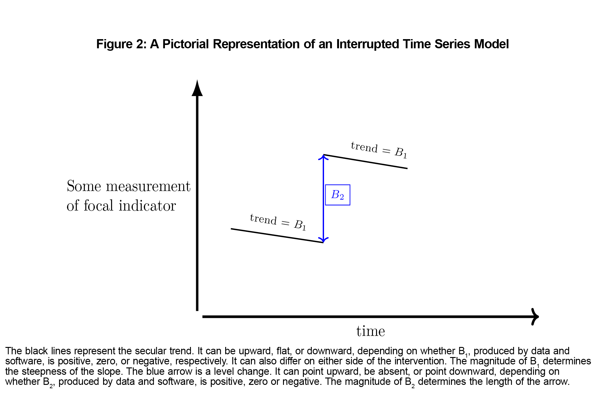
Like most statistical modeling, ITS analysis produces numerical results that represent real-world phenomena. Figure 2 shows the substantive meaning of typical output from a simple ITS model.

Absent a control setting, Bradford Hill’s criteria for assessing possible causation from observational studies can be applied to an ITS analysis.^9,10 When we have implemented an intervention and observed an improvement in a time series of our focal indicator, we are more confident that our intervention might be the cause when:

• The temporal sequence is correct. Improvements already underway cannot stem from the intervention.
• The improvement is large and unmistakable.
• The result is consistent when the intervention is implemented in other settings.
• There is a plausible mechanism, based on sound biopsychosocial or administrative theory. An improvement in the rate of colon cancer screening is unlikely to have been caused by the new coat of paint in the waiting room, whereas improvement in patient satisfaction scores might well have been.

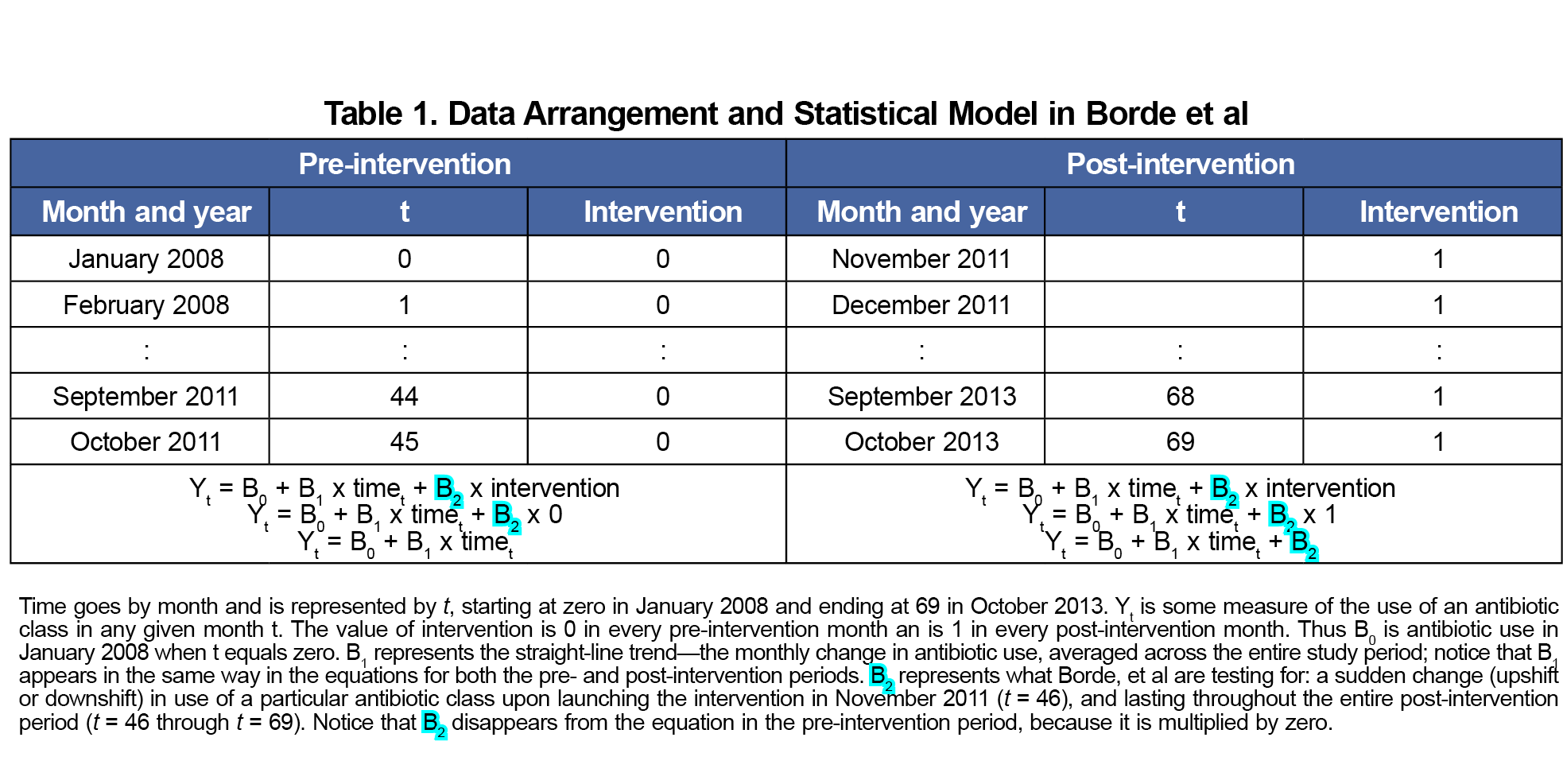
A study by Borde et al, provides an instructive example of ITS analysis that contains both strengths and weaknesses.¹¹ The investigators implemented a multifaceted intervention in the emergency department of a single academic medical center to increase the use of narrower rather than broader-spectrum antibiotics. The authors helpfully provided the equation representing their ITS model:

Y_t = B₀ + (B₁ × time_t) + (B₂ × intervention_t) + u_t                             (1)

u_t represents the inevitable random variation in the system; we will ignore it for now. Table 1 provides the details.

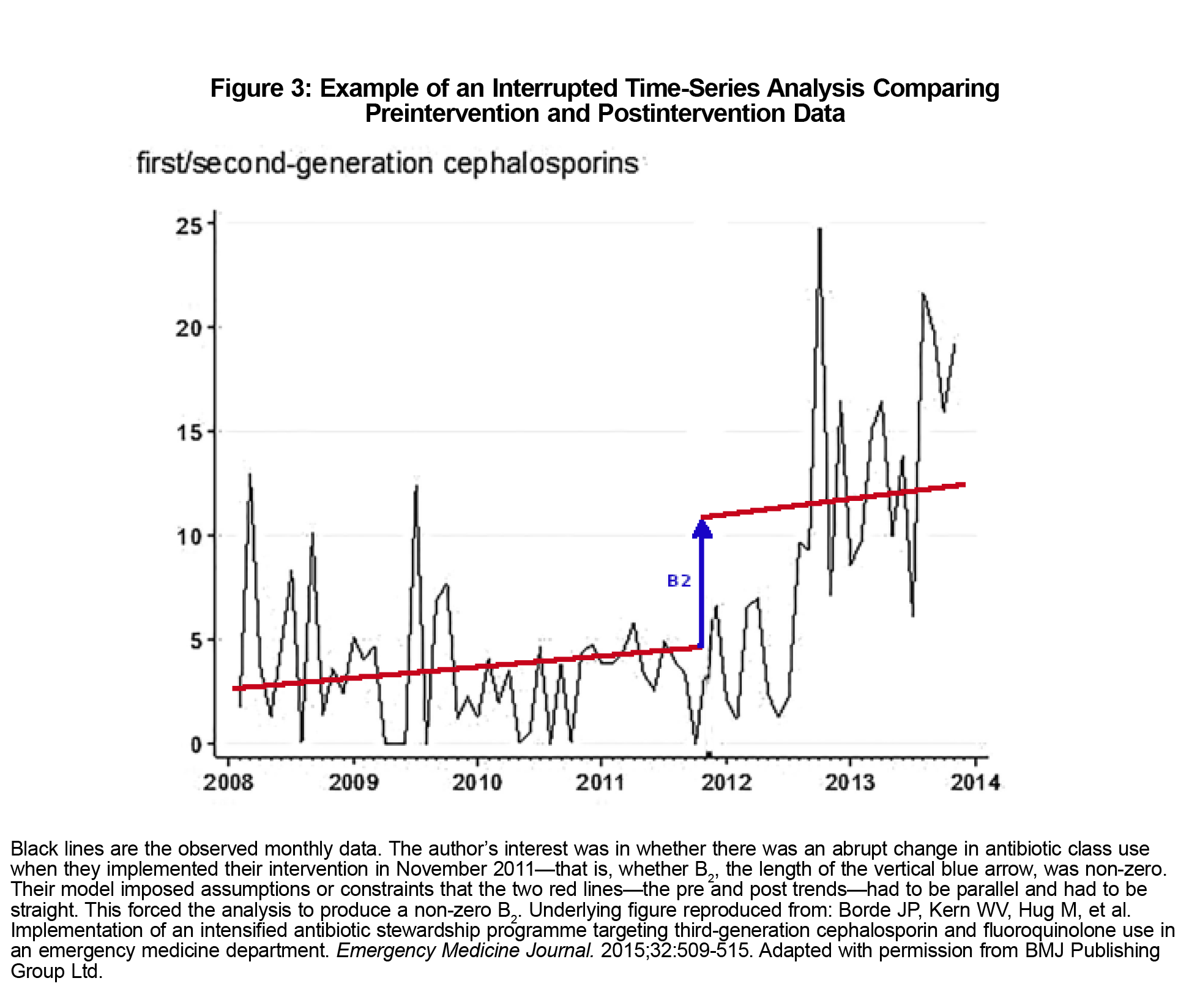
We will consider only their analysis of first- and second-generation cephalosporin use, which they hoped to preferentially increase. They hypothesized an abrupt increase in use upon implementing the intervention—a “level change.” In terms of the model represented by Equation 1, this is B₂, which statistical software will calculate based on sample data. B₂ significantly greater than zero would suggest that the intervention worked—the use of first- and second-generation cephalosporins increased abruptly when it was launched. Conversely, an estimate of B₂ that could plausibly be zero would suggest that it did not.

Borde et al controlled for a secular trend—that is B₁ in the model equation. They also controlled for autocorrelation (details not discussed here).

However, their model includes two consequential assumptions, or constraints, regarding the secular trend: (1) that it is the same before and after the intervention, and (2) that it is a straight line. Neither of these assumptions is required, and in this example the conclusion—that there was an abrupt increase in first- and second-generation cephalosporin use—is likely an artifact of those two assumptions, as shown in Figure 3.

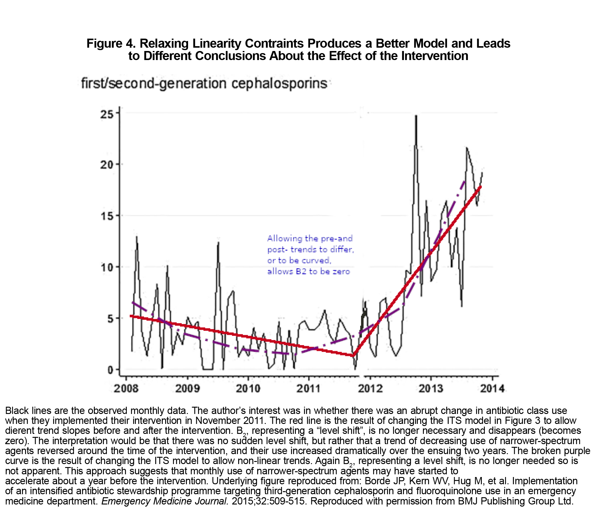
Relaxing the first assumption and allowing the slope of the trend line to differ before and after the intervention fits the observed data much better. This model would have led to a different conclusion: that there was no level change, but rather a dramatic reversal of what had been a gradual decrease in the use of the narrower-spectrum agents. Relaxing the second assumption and allowing trends to be curved would again have shown no level change, but rather a reversal in the decreasing use of narrower-spectrum agents beginning a year before the intervention (Figure 4). While perhaps just as clinically gratifying, these are different conclusions from those reached by the authors.

The passage of time is inevitable and can affect outcomes of interest. Pre/post QI studies do not adequately control for trends arising from the passage of time. Interrupted time series modeling, the QI intervention being the “interruption,” provides a more robust, informative, and flexible approach.

The ITS example explored in detail here serves also as a reminder that all statistical tests and models entail assumptions, some of them chosen by the analysts. To interpret findings, it is important to understand the constraints imposed by the model used. In ITS, it is generally best to allow for the possibility of nonlinear trends that differ pre- and post-intervention.

References

- Brady PW, Tchou MJ, Ambroggio L, Schondelmeyer AC, Shaughnessy EE. Quality improvement feature series article 2: displaying and analyzing quality improvement data. J Pediatric Infect Dis Soc. 2018;7(2):100-103. doi:10.1093/jpids/pix077
- Chen YF, Hemming K, Stevens AJ, Lilford RJ. Secular trends and evaluation of complex interventions: the rising tide phenomenon. BMJ Qual Saf. 2016;25(5):303-310. doi:10.1136/bmjqs-2015-004372
- Ryan CW. Decreased respiratory-related absenteeism among preschool students after installation of upper room germicidal ultraviolet light: analysis of newly discovered historical data. Int J Environ Res Public Health. 2023; 20.3:2536.doi:10.3390/ijerph20032536.
- Irazola V et al. Quality improvement intervention to increase colorectal cancer screening at the primary care setting: a cluster-randomised controlled trial. BMJ Open Quality. 2023; 12.2:e002158.doi:10.1136/bmjoq-2022-002158
- Hullick C, Conway J, Higgins I, et al. Emergency department transfers and hospital admissions from residential aged care facilities: a controlled pre-post design study. BMC Geriatr. 2016;16(1):102. doi:10.1186/s12877-016-0279-1
- Lee TC, Murray J, McDonald EG. An online educational module on transfusion safety and appropriateness for resident physicians: a controlled before-after quality-improvement study. CMAJ Open. 2019;7(3):E492-E496. doi:10.9778/cmajo.20180211
- ALMohiza MA, Sparto PJ, Marchetti GF, et al. A quality improvement project in balance and vestibular rehabilitation and its effect on clinical outcomes. J Neurol Phys Ther. 2016;40(2):90-99. doi:10.1097/NPT.0000000000000125
- Tarabichi Y, Cheng A, Bar-Shain D, et al. Improving timeliness of antibiotic administration using a provider and pharmacist facing sepsis early warning system in the emergency department setting: a randomized controlled quality improvement initiative. Crit Care Med. 2022;50(3):418-427. doi:10.1097/CCM.0000000000005267
- Hill AB. The environment and disease: association or causation? Proc R Soc Med. 1965;58(5):295-300. doi:10.1177/003591576505800503
- Poots AJ, Reed JE, Woodcock T, Bell D, Goldmann D. How to attribute causality in quality improvement: lessons from epidemiology. BMJ Qual Saf. 2017;26(11):933-937. doi:10.1136/bmjqs-2017-006756
- Borde JP, Kern WV, Hug M, et al. Implementation of an intensified antibiotic stewardship programme targeting third-generation cephalosporin and fluoroquinolone use in an emergency medicine department. Emerg Med J. 2015;32(7):509-515. doi:10.1136/emermed-2014-204067
There are no comments for this article.